مهندس باش !

سلام دوستان

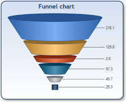
در ادامه آموزش های زبان انگلیسی ، آموزش ساخت نمودار قیفی رو شاهد خواهیم بود

There are several steps to create a funnel chart, please follow step by step.

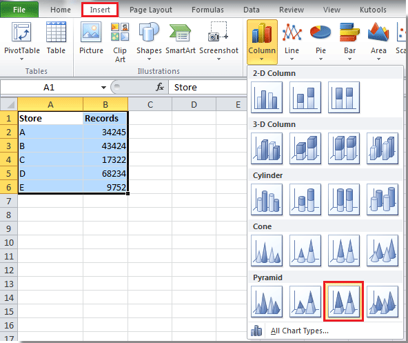
1. Select the data range and click Insert > Column > 100% Stacked Pyramid. See screenshot:

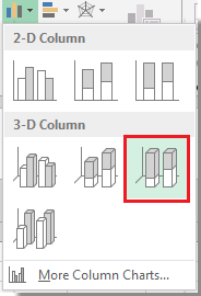
Tip: In Excel 2013, do as follow to insert 100% Stacked Pyramid.

(1).You need to insert a 3-D 100% Stacked Column first. Click Insert > Column > 3-D 100%Stacked Column. See screenshot:

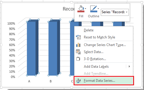
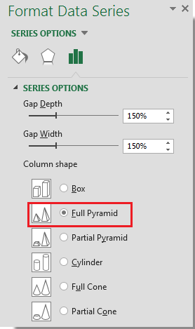
(2).And then right click at the column chart series to select Format Data Series, and check Full Pyramid option. See screenshots:

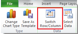
2. Click at the chart, and click Design > Switch Row/Column in the Data group. See screenshot:

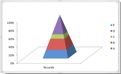
Now you can see the chart as shown as below:

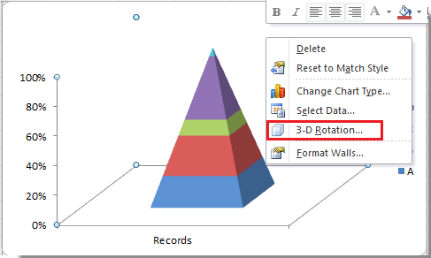
3. Right click the chart to select 3-D Rotation in the context menu. See screen shot:

4. In the Format Chart Area dialog, change the values in X and Y text boxes to zero in the Rotation section, and close this dialog. See screenshot:

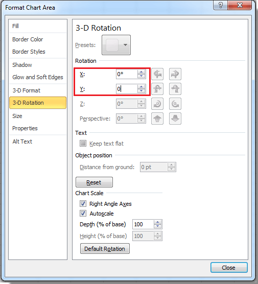
In Excel 2013 change the values in X and Y text boxes to zero in the 3-D Rotation section in the Format Chart Area pane.

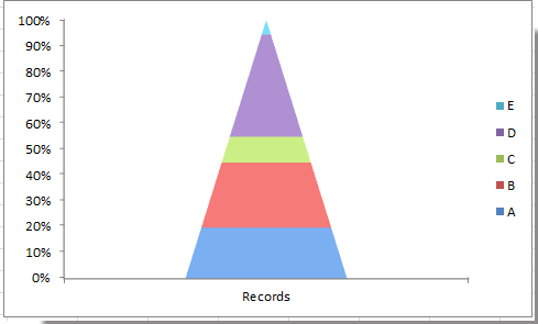
Now the chart change to this:

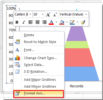
5. Right click at the Y axis and select Format Axis, then check Values in reverse order option. See screenshots:

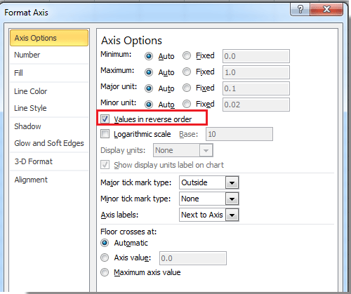In Excel 2013 check Values in reverse order in Format Axis pane.

6. Close the dialog. And you can delete axis, legend, and chart floor as you need, and also you can add the data labels in the chart by right click at the series and select Add Data Labels one by one.

Now you can see a completed funnel chart.