مهندس باش !

برای این پست آموزش ساخت نمودار Bullet یا همون ساختن رو ارایه داریم

Bullet chart is also named as build up chart in Excel, please follow the below steps to create it.

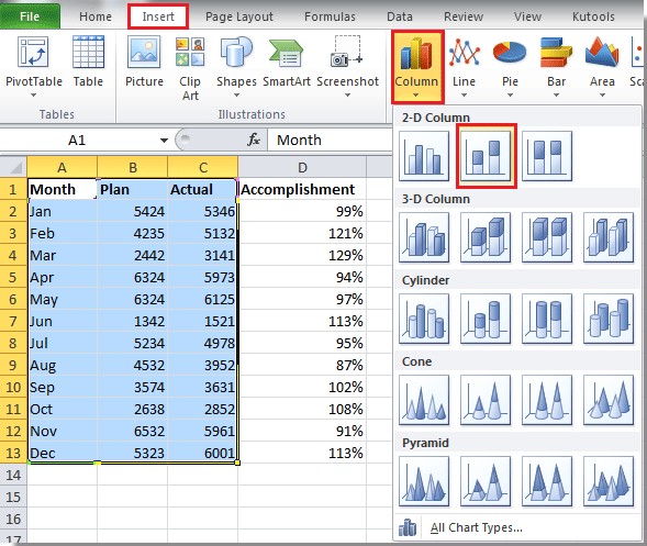
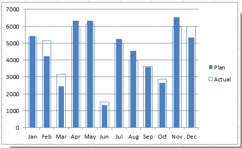
1. Select the data range excluding Accomplishment column, then click Insert > Column > Sacked Column. See screenshot:

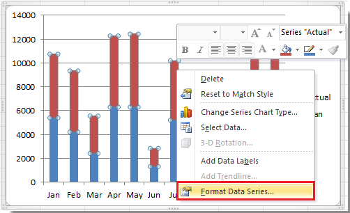
2. In the inserted column, right click at the Actual series and select Format Data Series from the context menu. See screenshot:

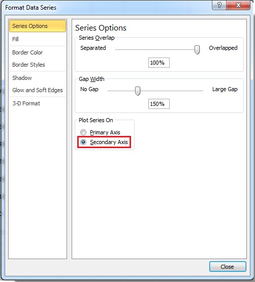
3. In the Format Data Series dialog, check Secondary Axis option. See screenshot:

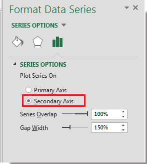
In Excel 2013, check Secondary Axis under SERIES OPTIONS section in the Format Data Series pane. See screenshot:

4. Close the dialog. Then select the secondary axis in the chart, and press Delete key on the keyboard to delete it. See screenshot:

5. Select the Actual series again, and right click to select Format Data Series.

6. In the Format Data Series dialog, do as follow:

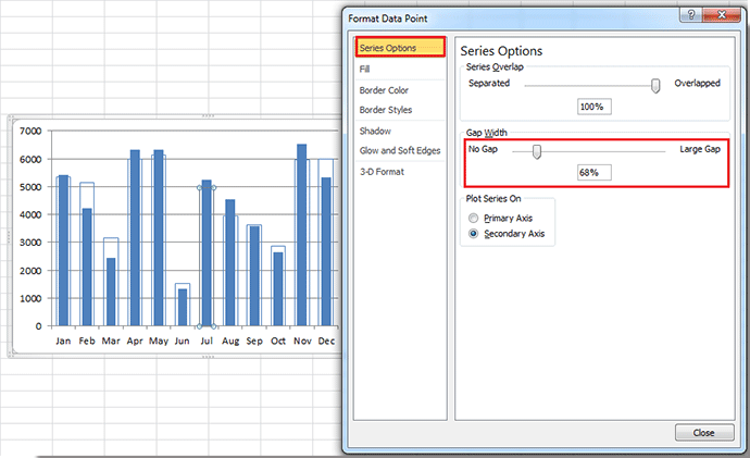
(1) Click Series Options tab, and adjust the gap width until the Actual series width is wider than Plan series. See screenshot:

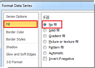
(2) Click Fill tab, and check No fill option. See screenshot:

(3) Click Border Color tab, check Solid line option. See screenshot:

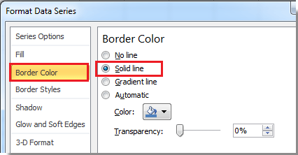
In Excel 2013, you need to adjust gap width under Series Options tab, check No fill option and Solid line option in Fill section and Border section under Fill & Line tab.

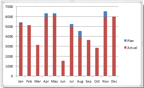
7. Close the dialog, you can see the bullet chart has been completed in the main.

Now you can add the Accomplish percentage at the top of the series.

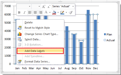
8. Right click at one series, and select Add Data Labels. See screenshot:

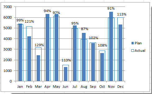
9. Then type the percentage value into the data label text box and drag them to the top of the series one by one. Now you can see the final chart: